30 Excel formulas and functions with examples and Copilot prompts

Accurate, reliable data starts with the right spreadsheet foundations. Reduce manual errors, catch mistakes early, and build logic that holds up every time data changes using Microsoft Excel formulas and functions. From simple totals to cross-table lookups, each formula is built into Excel for the web and ready to use with no installation required.

Explore 30 essential Excel formulas and functions, ranging from data clean up to analysis. Review step-by-step guidance and real-world scenarios to learn each function, or use Copilot in Excel prompt examples to build the formula from a description using AI.

Clean data for analysis

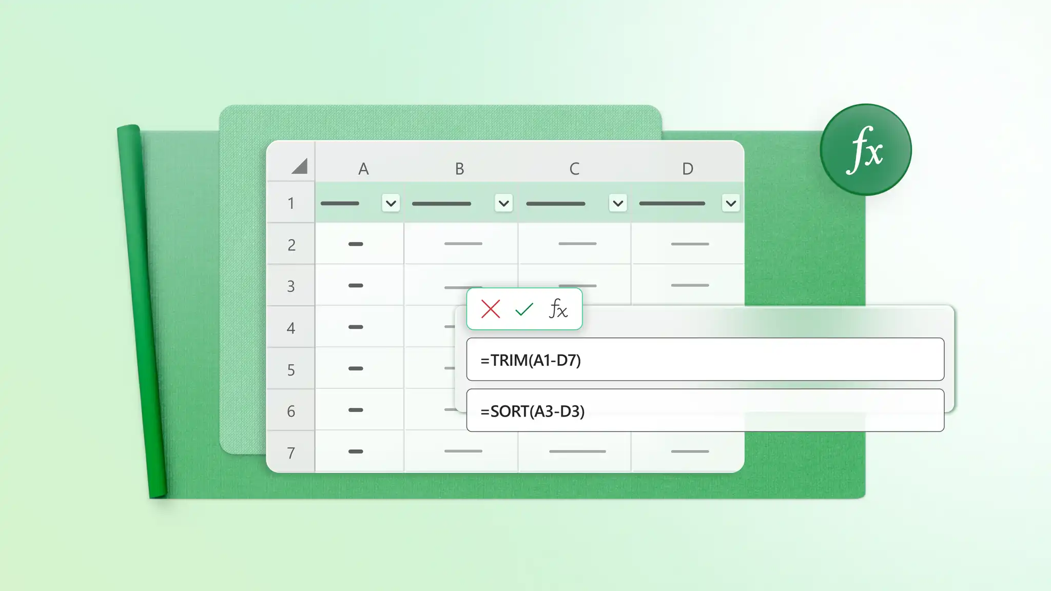
Getting data into a consistent, usable state is the first step before running any calculation. Use these formulas to remove extra spaces, combine or split text, and standardize imported data, so that formulas, lookups, charts, and PivotTables produce reliable results.

TRIM

TRIM removes extra spaces from the start, end, and between words in a text string, leaving only single spaces between words.

How to use TRIM

1. Select an empty cell next to the text you want to clean.

2. Type =TRIM(A2).

3. Press Enter and fill the formula down the column.

When to use TRIM

• Cleaning customer names imported from another system

• Fixing spacing issues that break XLOOKUP or COUNTIF formulas

• Standardizing product IDs and text fields

Try this Copilot prompt"Clean this column by removing extra spaces and standardizing text formatting."Click to copy this Copilot prompt

CONCAT and TEXTJOIN 

CONCAT and TEXTJOIN combine values from multiple cells into a single text string. TEXTJOIN adds a chosen separator between values.

How to use CONCAT and TEXTJOIN

1. Select the cell where the combined text should appear.

2. Enter a CONCAT or TEXTJOIN formula with the cells to join.

3. Press Enter to create the combined value.

When to use CONCAT and TEXTJOIN

• Combining first and last names

• Building full addresses from separate columns

• Creating product labels or display names

Try this Copilot prompt"Combine the values in columns A, B, and C into a single address using TEXTJOIN."Click to copy this Copilot prompt

LEFT and RIGHT

LEFT pulls a set number of characters from the start of a text string, and RIGHT pulls them from the end, such as the first 3 characters of a product code or the last 4 digits of a phone number.

How to use LEFT and RIGHT

1. Select the cell where the result should appear.

2. Type =LEFT(A2,3) or =RIGHT(A2,3).

3. Press Enter to return the required characters.

When to use LEFT and RIGHT

• Pulling a region or branch code off the front of a product ID

• Isolating a file extension or the last digits of a reference number

• Separating a fixed-length prefix from the rest of an identifier

Try this Copilot prompt"Extract the first three characters from every product ID in this table."Click to copy this Copilot prompt

SORT

SORT produces a reordered copy of a range in a new location, leaving the original data untouched.

How to use SORT

1. Select an empty area of the worksheet.

2. Enter a SORT formula using your source range.

3. Press Enter to create a dynamically sorted list.

When to use SORT

• Reordering a project task list by due date without disturbing the source

• Reviewing an inventory tracker from lowest to highest stock level

• Arranging records into rank order before a review or report

Try this Copilot prompt"Create a SORT formula that returns tasks ordered by due date."Click to copy this Copilot prompt

FILTER

FILTER returns only the rows from a range that meet a defined condition, updating automatically as the source changes.

How to use FILTER

1. Select an empty area of the worksheet.

2. Enter a FILTER formula and define the condition.

3. Press Enter to display matching records.

When to use FILTER

• Pulling just the active accounts out of a full client list

• Showing only overdue items from a project tracker

• Isolating a single month of entries from a full-year dataset

Try this Copilot prompt"Create a FILTER formula that shows only rows where the status column equals Active."Click to copy this Copilot prompt

UNIQUE

UNIQUE returns a list of distinct values from a range, removing repeated entries from the result.

How to use UNIQUE

1. Select an empty cell where the unique list should appear.

2. Enter a UNIQUE formula and select the range you want to pull distinct values from.

3. Press Enter to return each distinct value from the source range.

When to use UNIQUE

• Creating a list of unique customers or products in a business

• Removing repeated names from a signup list or attendance sheet

• Building category lists for reporting or analysis

Try this Copilot prompt"Create a formula that returns a list of unique values from the customer column."Click to copy this Copilot prompt

TEXTSPLIT

TEXTSPLIT separates text using a comma, space, or hyphen, into distinct columns or rows.

How to use TEXTSPLIT

1. Select an empty cell next to the text you want to split.

2. Enter a TEXTSPLIT formula with the source cell and delimiter.

3. Press Enter to split the text into separate cells.

When to use TEXTSPLIT

• Separating full names into first and last names

• Splitting comma-separated tags or categories

• Breaking product codes into separate components

Try this Copilot prompt"Split the full names in column A into first name and last name columns."Click to copy this Copilot prompt

Calculate totals and averages

Use calculation formulas to answer everyday spreadsheet questions, including totals, averages, counts, and rankings.

SUM

SUM adds every value in a selected range or set of cells.

How to use SUM

1. Select the cell where the total should appear.

2. Enter a SUM formula and select the range of cells you want to total.

3. Press Enter to calculate the total.

When to use SUM

• Adding monthly expenses in a budget planner

• Calculating total business revenue

• Summing hours, units, or quantities

Try this Copilot prompt"Create a SUM formula that adds all values in the revenue column."Click to copy this Copilot prompt

AVERAGE

AVERAGE calculates the mean value across a selected range.

How to use AVERAGE

1. Select the cell where the average should appear.

2. Enter an AVERAGE formula and select the range you want to average.

3. Press Enter to calculate the average.

When to use AVERAGE

• Finding average order value over a quarter

• Calculating average response times across a team

• Reviewing average weekly hours or costs

Try this Copilot prompt"Create a formula that calculates the average value in the monthly spend column."Click to copy this Copilot prompt

MIN and MAX

MIN returns the smallest value in a range, and MAX returns the largest value.

How to use MIN and MAX

1. Select an empty cell for the result.

2. Enter a MIN or MAX formula and select the range of values to check.

3. Press Enter to return the lowest or highest value.

When to use MIN and MAX

• Spotting outliers in an expense reports

• Checking that data entry stays within expected bounds

• Surfacing the best and worst performers in a sales column

Try this Copilot prompt"Find the highest and lowest values in the sales column using MIN and MAX formulas."Click to copy this Copilot prompt

COUNT and COUNTA

COUNT tallies cells that contain numbers, while COUNTA counts any cell that is not blank.

How to use COUNT and COUNTA

1. Select the cell where the count should appear.

2. Enter a COUNT formula to count numbers, or a COUNTA formula to count non-blank cells.

3. Select the range you want to count, then press Enter.

When to use COUNT and COUNTA

• Counting numeric entries in a revenue column

• Counting completed fields in a tracker

• Checking how many rows contain data

Try this Copilot prompt"Count how many rows have values in this table and explain whether COUNT or COUNTA is the better formula."Click to copy this Copilot prompt

COUNTIF

COUNTIF counts cells that meet a single condition.

How to use COUNTIF

1. Select the cell where the result should appear.

2. Enter a COUNTIF formula with the range and condition.

3. Press Enter to count matching cells.

When to use COUNTIF

• Counting invoices marked Paid

• Counting orders from one region

• Counting responses with a specific status or category

Try this Copilot prompt"Create a COUNTIF formula that counts how many tasks are marked Complete."Click to copy this Copilot prompt

SUMIF

SUMIF adds values that meet a single condition.

How to use SUMIF

1. Select the cell where the total should appear.

2. Enter a SUMIF formula with the criteria range, condition, and sum range.

3. Press Enter to calculate the conditional total.

When to use SUMIF

• Adding sales from one channel

• Totaling expenses in one category

• Calculating timesheet hours for one project or client

Try this Copilot prompt"Create a SUMIF formula that totals sales only where the channel column equals Online."Click to copy this Copilot prompt

RANK.EQ

RANK.EQ returns the position of a number within a list, from highest to lowest or the reverse.

How to use RANK.EQ

1. Select an empty cell next to the value you want to rank.

2. Enter a RANK.EQ formula with the value and comparison range.

3. Press Enter and fill the formula down the column.

When to use RANK.EQ

• Ranking salespeople by revenue

• Ordering marketing campaign results by conversion rate

• Identifying top-performing products or regions

Try this Copilot prompt"Rank each sales value from highest to lowest using a RANK.EQ formula."Click to copy this Copilot prompt

Use logic and handle errors in formulas

Logic formulas help a spreadsheet respond to different conditions. Use them to show different results based on the data, combine multiple rules into one test, or keep formulas readable when an Excel error appears.

IF

IF returns one result when a condition is true and another result when it is false.

How to use IF

1. Select the cell where the result should appear.

2. Enter an IF formula with a condition, a true result, and a false result.

3. Press Enter to return the matching result.

When to use IF

• Marking tasks as On track or Needs review

• Labeling scores as Above target or Below target

• Flagging invoices as Paid or Overdue

Try this Copilot prompt"Create an IF formula that shows On track when the value in column B is above 80%, and Needs review when it is not."Click to copy this Copilot prompt

IFERROR

IFERROR catches any error a formula returns and replaces it with a specified value, such as a dash, a zero, or a plain-language note.

How to use IFERROR

1. Select the cell where the formula result should appear.

2. Wrap the original formula in IFERROR.

3. Add the value or message to show if an error appears.

When to use IFERROR

• Replacing lookup errors with a blank cell or message

• Keeping reports readable when data is missing

• Avoiding visible formula errors in shared sheets

Try this Copilot prompt"Wrap this lookup formula in IFERROR so it shows Not found when there is no matching result."Click to copy this Copilot prompt

AND and OR

AND checks whether all conditions are true, while OR checks whether at least one condition is true.

How to use AND and OR

1. Select the cell where the logic result should appear.

2. Enter an AND or OR formula with the conditions to test.

3. Use the formula alone or inside IF for a custom result.

When to use AND and OR

• Checking whether multiple approval conditions are met

• Flagging records that match one of several categories

• Building more precise IF formulas

Try this Copilot prompt"Create a formula that marks a task as Ready only when the status is Complete and the approval column says Yes."Click to copy this Copilot prompt

SWITCH

SWITCH compares one value against a list of options and returns the matching result.

How to use SWITCH

1. Select the cell where the result should appear.

2. Enter a SWITCH formula with the value to check and possible matches.

3. Add a default result for values that do not match.

When to use SWITCH 

• Converting short status codes into full labels

• Assigning categories based on a single field

• Replacing long nested IF formulas with a cleaner option

Try this Copilot prompt"Create a SWITCH formula that converts status codes into labels such as Not started, In progress, Complete, and Blocked."Click to copy this Copilot prompt

Find and match information across datasets

Lookup formulas connect related information across tables. Use them to match IDs, retrieve values, or find the position of an item without manually scanning rows.

XLOOKUP

XLOOKUP can search a range in any direction and returns a related value, and it can return a set value when no match is found.

How to use XLOOKUP

1. Select the cell where the matching result should appear.

2. Enter an XLOOKUP formula with the lookup value, lookup range, and return range.

3. Press Enter to return the matching value.

When to use XLOOKUP

• Matching order IDs to customer names

• Pulling prices from a product list

• Returning values from tables where the lookup column is not first

Try this Copilot prompt"Create an XLOOKUP formula that matches the product ID in column A with the product name in another table."Click to copy this Copilot prompt

VLOOKUP

VLOOKUP can search the first column of a table from left to right and returns a value from a specified column in the same row.

How to use VLOOKUP

1. Select the cell where the matching result should appear.

2. Enter a VLOOKUP formula with the lookup value, table range, column number, and match type.

3. Press Enter to return the matching value.

When to use VLOOKUP

• Working with older or shared spreadsheets

• Matching IDs to values in a simple table

• Looking up information from left to right

Try this Copilot prompt"Create a VLOOKUP formula that matches each employee ID with the employee name from the lookup table."Click to copy this Copilot prompt

MATCH

MATCH returns the position of a value in a list, such as finding that an inventory product name is the 3rd item in a column.

How to use MATCH

1. Select the cell where the position should appear.

2. Enter a MATCH formula with the lookup value and lookup range.

3. Press Enter to return the item position.

When to use MATCH

• Finding where a value appears in a list

• Locating column positions in a table

• Pairing with INDEX for flexible lookups

Try this Copilot prompt"Create a MATCH formula that finds the position of the selected product code in this list."Click to copy this Copilot prompt

INDEX

INDEX retrieves a value from a specific position in a range or table.

How to use INDEX

1. Select the cell where the result should appear.

2. Enter an INDEX formula with the array, row number, and column number.

3. Press Enter to return the value at that position.

When to use INDEX

• Returning a value from a known row and column

• Building flexible lookup formulas with MATCH

• Pulling values from columns to the left of the search column, where VLOOKUP cannot reach

Try this Copilot prompt"Create an INDEX and MATCH formula that returns the price for each product code."Click to copy this Copilot prompt

Analyze and summarize large datasets

Use these formulas to calculate values across multiple conditions, summarize filtered lists, and compare averages across categories. They turn large tables into focused results without changing the source data.

SUMIFS

SUMIFS adds up the values in a column that satisfy two or more conditions at the same time.

How to use SUMIFS

1. Select the cell where the result should appear.

2. Enter a SUMIFS formula with the sum range first.

3. Add each criteria range and its condition.

When to use SUMIFS

• Totaling revenue for one product in one region

• Adding the hours one employee logged in a specific week

• Summing expenses in a single category for a single month

Try this Copilot prompt"Calculate total revenue for Product A in Region B using a SUMIFS formula."Click to copy this Copilot prompt

SUBTOTAL

SUBTOTAL calculates results such as sums, averages, and counts for a filtered list, using only the visible rows.

How to use SUBTOTAL

1. Select the cell where the summary should appear.

2. Enter a SUBTOTAL formula with the function number and range.

3. Apply filters to the table to update the visible result.

When to use SUBTOTAL

• Summarizing only visible rows in a filtered list

• Reviewing totals after applying filters

• Creating quick summaries without changing the source data

Try this Copilot prompt"Create a SUBTOTAL formula that sums only the visible rows in this filtered table."Click to copy this Copilot prompt

AVERAGEIF

AVERAGEIF calculates the average of values that meet a single condition.

How to use AVERAGEIF

1. Select the cell where the average should appear.

2. Enter an AVERAGEIF formula with the criteria range, condition, and average range.

3. Press Enter to calculate the conditional average.

When to use AVERAGEIF

• Finding average sales for one product

• Calculating average spend by category

• Reviewing average scores for one group

Try this Copilot prompt"Create an AVERAGEIF formula that calculates the average order value for customers in the East region."Click to copy this Copilot prompt

Work with dates and deadlines

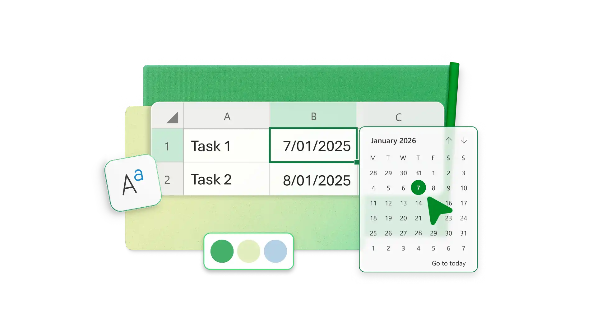
Date formulas calculate deadlines, measure time between events, and keep schedules current. Use them to track tasks, review timelines, and build reports that update as dates change.

TODAY

TODAY returns the current date and updates each time the workbook recalculates.

How to use TODAY

1. Select the cell where the current date should appear.

2. Enter a TODAY formula, which takes no arguments.

3. Press Enter to display today's date.

When to use TODAY

• Calculating days until a deadline

• Marking overdue tasks

• Creating reports that update based on the current date

Try this Copilot prompt"Create a formula that compares each due date with today's date and marks overdue tasks."Click to copy this Copilot prompt

DATEDIF

DATEDIF calculates the difference between two dates in days, months, or years according to the calendar.

How to use DATEDIF

1. Select the cell where the date difference should appear.

2. Enter a DATEDIF formula with the start date, end date, and unit.

3. Press Enter to return the time between the dates.

When to use DATEDIF

• Calculating student assignment durations

• Finding days between request and completion dates

• Measuring age, tenure, or time elapsed

Try this Copilot prompt"Create a DATEDIF formula that calculates how many days each project took from start date to completion date."Click to copy this Copilot prompt

WORKDAY

WORKDAY returns a date before or after a range of working days, and can exclude weekends and holidays.

How to use WORKDAY

1. Select the cell where the deadline should appear.

2. Enter a WORKDAY formula with the start date and number of workdays.

3. Add holidays if the schedule should exclude them.

When to use WORKDAY

• Calculating project due dates

• Scheduling follow-up dates

• Planning timelines that exclude weekends

Try this Copilot prompt"Create a WORKDAY formula that adds ten working days to each start date and excludes weekends."Click to copy this Copilot prompt

Use Copilot in Excel to create and understand formulas

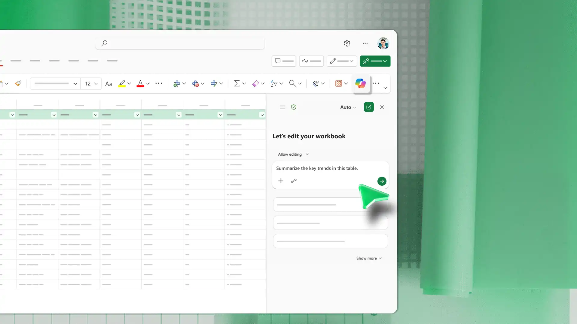
Copilot helps generate formulas from plain-language instructions as well as identify the cause of formula errors in Excel. The AI spreadsheet assistant provides suggestions, so reviewing results before applying them to an important workbook remains essential. Here are some ways to use Copilot:

• Ask Copilot to explain an unfamiliar formula in everyday terms in the chat.

• Describe the calculation needed in Copilot chat and let Copilot suggest a formula. Review the suggested formula before adding it to a shared or high-impact spreadsheet.

• Request Copilot to diagnose errors like broken formulas or missing spreadsheet formatting.

Note: working with Copilot in Excel requires either a Microsoft 365 Personal or Family subscription (with an AI credits plan (opens in a new tab)), a Microsoft 365 Premium (opens in a new tab) subscription, or a commercial Microsoft 365 Copilot subscription (opens in a new tab).

With the right formulas, Excel spreadsheet maker can organize messy data, calculate values, check conditions, match information, and summarize large tables efficiently. Use this guide to start with the formulas that match the task at hand, or use Copilot in Excel to explore formula options to complete tasks with AI.